Pandas Tutorial

import numpy as np
import pandas as pd


import matplotlib.pyplot as plt

pd.options.display.max_columns = 50

Series

Series are one-dimensional objects like lists, numpy arrays or table columns. Each series has an index that can be used to find elements. By default this is an integer from 0 to n-1.

values = [3, "foo", 3.14, 42, -23, "bar"]

s = pd.Series(values)

print(s)

0       3
1     foo
2    3.14
3      42
4     -23
5     bar
dtype: object

s[3]

index = ["a", "b", "c", "d", "e", "f"]

s = pd.Series(values, index=index)

a       3
b     foo
c    3.14
d      42
e     -23
f     bar
dtype: object

s["d"]

s[["a", "b", "c"]]

a       3
b     foo
c    3.14
dtype: object

s = pd.Series(np.arange(10), index=np.arange(10, 20))
s[s > 5]

16    6
17    7
18    8
19    9
dtype: int64

DataFrames

Are two-dimensional data structures similar to tables or Excel sheets. Basically a collection of Series. We use the table of the largest cities in Europe from wikipedia as an example here.

cities_url = "https://en.wikipedia.org/wiki/List_of_largest_cities"
tables = pd.read_html(cities_url, header=0, flavor="bs4")

df = tables[1]

df.info()

<class 'pandas.core.frame.DataFrame'>
RangeIndex: 83 entries, 0 to 82
Data columns (total 13 columns):
 #   Column                           Non-Null Count  Dtype 
---  ------                           --------------  ----- 
 0   City[a]                          82 non-null     object
 1   Country                          82 non-null     object
 2   UN 2018 population estimates[b]  82 non-null     object
 3   City proper[c]                   82 non-null     object
 4   City proper[c].1                 82 non-null     object
 5   City proper[c].2                 82 non-null     object
 6   City proper[c].3                 82 non-null     object
 7   Urban area[8]                    82 non-null     object
 8   Urban area[8].1                  82 non-null     object
 9   Urban area[8].2                  82 non-null     object
 10  Metropolitan area[d]             82 non-null     object
 11  Metropolitan area[d].1           82 non-null     object
 12  Metropolitan area[d].2           82 non-null     object
dtypes: object(13)
memory usage: 8.6+ KB

df.memory_usage(deep=True)

Index                               132
City[a]                            4711
Country                            4621
UN 2018 population estimates[b]    4681
City proper[c]                     5302
City proper[c].1                   4727
City proper[c].2                   4462
City proper[c].3                   4945
Urban area[8]                      4690
Urban area[8].1                    4381
Urban area[8].2                    4493
Metropolitan area[d]               5269
Metropolitan area[d].1             5101
Metropolitan area[d].2             5236
dtype: int64

Method Chaining

df = (df.dropna()
        .rename(columns=df.iloc[0]).drop(df.index[0])
        .rename(columns=str.lower)
        .reset_index()      
        .rename(columns={"city[a]": "name", "index": "rank"})      
        .assign(country=lambda x: pd.Categorical(x["country"]),
                name=lambda x: pd.Categorical(x["name"]),
                population_est=lambda x: x["un 2018 population estimates[b]"].astype(np.int32),
                definition=lambda x: pd.Categorical(x["definition"]),
                density=lambda x: x["density (/km2)"].iloc[:, 0].str.replace(",", "").str.extract(r'(\d+)').astype(np.float32),
                rank=lambda x: x["rank"] - 1
        )
)[["rank", "name", "country", "definition", "population_est", "density"]]

df.info()

<class 'pandas.core.frame.DataFrame'>
RangeIndex: 81 entries, 0 to 80
Data columns (total 6 columns):
 #   Column          Non-Null Count  Dtype   
---  ------          --------------  -----   
 0   rank            81 non-null     int64   
 1   name            81 non-null     category
 2   country         81 non-null     category
 3   definition      81 non-null     category
 4   population_est  81 non-null     int32   
 5   density         74 non-null     float32 
dtypes: category(3), float32(1), int32(1), int64(1)
memory usage: 6.9 KB

df.head()

	rank	name	country	definition	population_est	density
0	1	Tokyo	Japan	Metropolis prefecture	37468000	6169.0
1	2	Delhi	India	Municipal corporation	28514000	11289.0
2	3	Shanghai	China	Municipality	25582000	3922.0
3	4	São Paulo	Brazil	Municipality	21650000	8055.0
4	5	Mexico City	Mexico	City-state	21581000	6202.0

df.sort_values(by="density", ascending=False).head()

	rank	name	country	definition	population_est	density
16	17	Manila	Philippines	Capital city	13482000	41399.0
8	9	Dhaka	Bangladesh	Capital city	19578000	26349.0
15	16	Kolkata	India	Municipal corporation	14681000	21935.0
6	7	Mumbai	India	Municipal corporation	19980000	20694.0
27	28	Paris	France	Commune	10901000	20460.0

Indices

Simple

ds = df.set_index("rank")

ds.loc[2:5, "country": "population_est"].head()

	country	definition	population_est
rank
2	India	Municipal corporation	28514000
3	China	Municipality	25582000
4	Brazil	Municipality	21650000
5	Mexico	City-state	21581000

ds.loc[ds.name.isin(("Paris", "Dhaka")), "country": "population_est"].head()

	country	definition	population_est
rank
9	Bangladesh	Capital city	19578000
28	France	Commune	10901000

Multidimensional

df.head()

	rank	name	country	definition	population_est	density
0	1	Tokyo	Japan	Metropolis prefecture	37468000	6169.0
1	2	Delhi	India	Municipal corporation	28514000	11289.0
2	3	Shanghai	China	Municipality	25582000	3922.0
3	4	São Paulo	Brazil	Municipality	21650000	8055.0
4	5	Mexico City	Mexico	City-state	21581000	6202.0

ds = df.set_index(["country", "definition", "rank"]).sort_index()

ds.loc["China",:,:]

		name	population_est	density
definition	rank
City (sub-provincial)	22	Guangzhou	12638000	1950.0
	25	Shenzhen	11908000	6111.0
	40	Chengdu	8813000	1116.0
	41	Nanjing	8245000	1103.0
	42	Wuhan	8176000	1282.0
	47	Xi'an	7444000	887.0
	50	Hangzhou	7236000	570.0
	52	Shenyang	6921000	639.0
	60	Harbin	6115000	200.0
	75	Qingdao	5381000	NaN
	76	Dalian	5300000	NaN
	80	Jinan	5052000	849.0
Municipality	3	Shanghai	25582000	3922.0
	8	Beijing	19618000	1334.0
	14	Chongqing	14838000	389.0
	20	Tianjin	13215000	1163.0
Prefecture-level city	49	Dongguan	7360000	3384.0
	51	Foshan	7236000	1870.0
	58	Suzhou	6339000	1263.0
Special administrative region	48	Hong Kong	7429000	6611.0

Simple Plots

size = (10, 5)

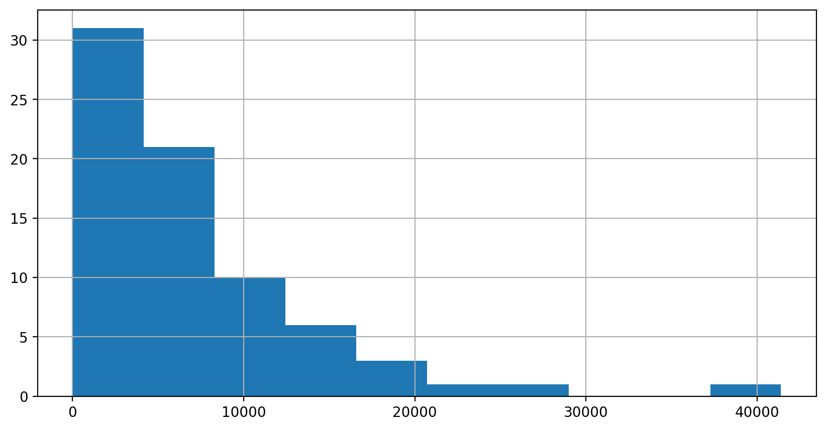
ax = df.density.hist(figsize=size)

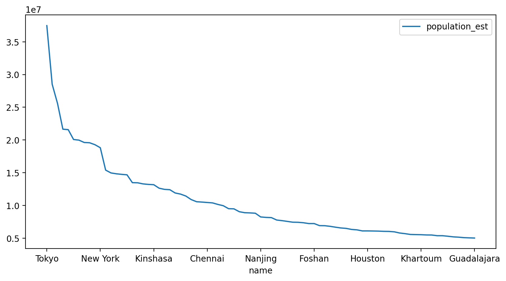
ax = df.plot(x="name", y="population_est", figsize=size)

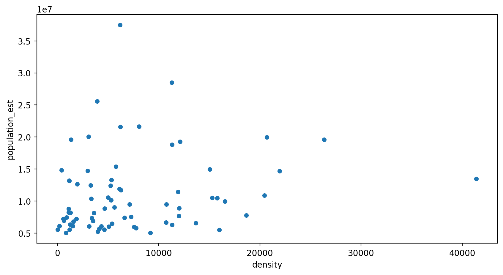
ax = df.plot.scatter(x="density", y="population_est", figsize=size)

Grouping

dt = (df[["country", "population_est", "name"]]
      .groupby("country", observed=False)
      .agg({"population_est": "sum", "name": "count"})
      .rename(columns={"name": "cities"})
      .reset_index()
      .sort_values(by="cities", ascending=False)
      .head(12))
dt

	country	population_est	cities
6	China	194846000	20
34	United States	74865000	9
11	India	115074000	9
15	Japan	71807000	4
3	Brazil	40915000	3
20	Pakistan	27138000	2
23	Russia	17793000	2
17	Mexico	26604000	2
9	Egypt	25162000	2
28	Spain	11991000	2
26	South Africa	5486000	1
24	Saudi Arabia	6907000	1

How often do which values occur in a column?

dt.cities.value_counts()

cities
2     5
9     2
1     2
20    1
4     1
3     1
Name: count, dtype: int64

Fetch the inhabitants per country

countries_url = "https://en.wikipedia.org/wiki/List_of_countries_and_dependencies_by_population"
tables = pd.read_html(countries_url, header=0, flavor="bs4", decimal=",", thousands=".")

dc = tables[0]

"1,34.5".replace(",.", "")

'1,34.5'

dc = (dc.rename(columns=str.lower)
   .assign(
       population=lambda x: x["population"].str.replace(r"[.,]", "", regex=True).astype(np.int64),
       country=lambda x: pd.Categorical(x["country / dependency"])
   )
)[["country", "population"]]

dc.head()

	country	population
0	World	8068346000
1	China	1411750000
2	India	1392329000
3	United States	335576000
4	Indonesia	279118866

query

dc.query("population > 10**6 and country in ('Niger', 'United States', 'India')")

	country	population
2	India	1392329000
3	United States	335576000
56	Niger	25369415

dt

	country	population_est	cities
6	China	194846000	20
34	United States	74865000	9
11	India	115074000	9
15	Japan	71807000	4
3	Brazil	40915000	3
20	Pakistan	27138000	2
23	Russia	17793000	2
17	Mexico	26604000	2
9	Egypt	25162000	2
28	Spain	11991000	2
26	South Africa	5486000	1
24	Saudi Arabia	6907000	1

Join - like in SQL

dm = (pd.merge(dt, dc, on="country")[["country", "cities", "population_est", "population"]]
        .rename(columns={"population_est": "in_cities", "population": "total"}))
dm

	country	cities	in_cities	total
0	China	20	194846000	1411750000
1	United States	9	74865000	335576000
2	India	9	115074000	1392329000
3	Japan	4	71807000	124340000
4	Brazil	3	40915000	203062512
5	Pakistan	2	27138000	241499431
6	Russia	2	17793000	146424729
7	Mexico	2	26604000	129202482
8	Egypt	2	25162000	105481000
9	Spain	2	11991000	48345223
10	South Africa	1	5486000	62027503
11	Saudi Arabia	1	6907000	32175224

dm["city_ratio"] = dm.in_cities / dm.total

dm

	country	cities	in_cities	total	city_ratio
0	China	20	194846000	1411750000	0.138017
1	United States	9	74865000	335576000	0.223094
2	India	9	115074000	1392329000	0.082649
3	Japan	4	71807000	124340000	0.577505
4	Brazil	3	40915000	203062512	0.201490
5	Pakistan	2	27138000	241499431	0.112373
6	Russia	2	17793000	146424729	0.121516
7	Mexico	2	26604000	129202482	0.205909
8	Egypt	2	25162000	105481000	0.238545
9	Spain	2	11991000	48345223	0.248029
10	South Africa	1	5486000	62027503	0.088445
11	Saudi Arabia	1	6907000	32175224	0.214668

Often used Operations

df = pd.DataFrame(index=["A", "B", "C"])
df["name"] = ["foo", "bar", "baz"]
df["value"] = [23, 42, 28]

df

	name	value
A	foo	23
B	bar	42
C	baz	28

df.reset_index()

	index	name	value
0	A	foo	23
1	B	bar	42
2	C	baz	28

dm = df.reset_index().melt(id_vars=["index"], value_name="new_value")
dm

	index	variable	new_value
0	A	name	foo
1	B	name	bar
2	C	name	baz
3	A	value	23
4	B	value	42
5	C	value	28

dm.pivot(columns="variable", values="new_value", index="index")

variable	name	value
index
A	foo	23
B	bar	42
C	baz	28